Bonding Curves and AMM Invariants: How Curve Shape Sets Risk

At its core, every pool you can put money into is a curve plus a fee.

The curve decides how much depth sits at each price. It decides how fast your holdings flip from one token to the other. And it decides which specific failure you are being paid to absorb. So picking a pool largely means picking a curve. One curve family goes further and moves itself to follow the market price; that design is unpacked in Curve v2 CryptoSwap Explained.

There are three basic shapes, and most real pools sit somewhere between them. By the end, you should be able to read an unfamiliar curve and say what it assumes, what it costs traders, and what it leaves you holding when the assumption fails.

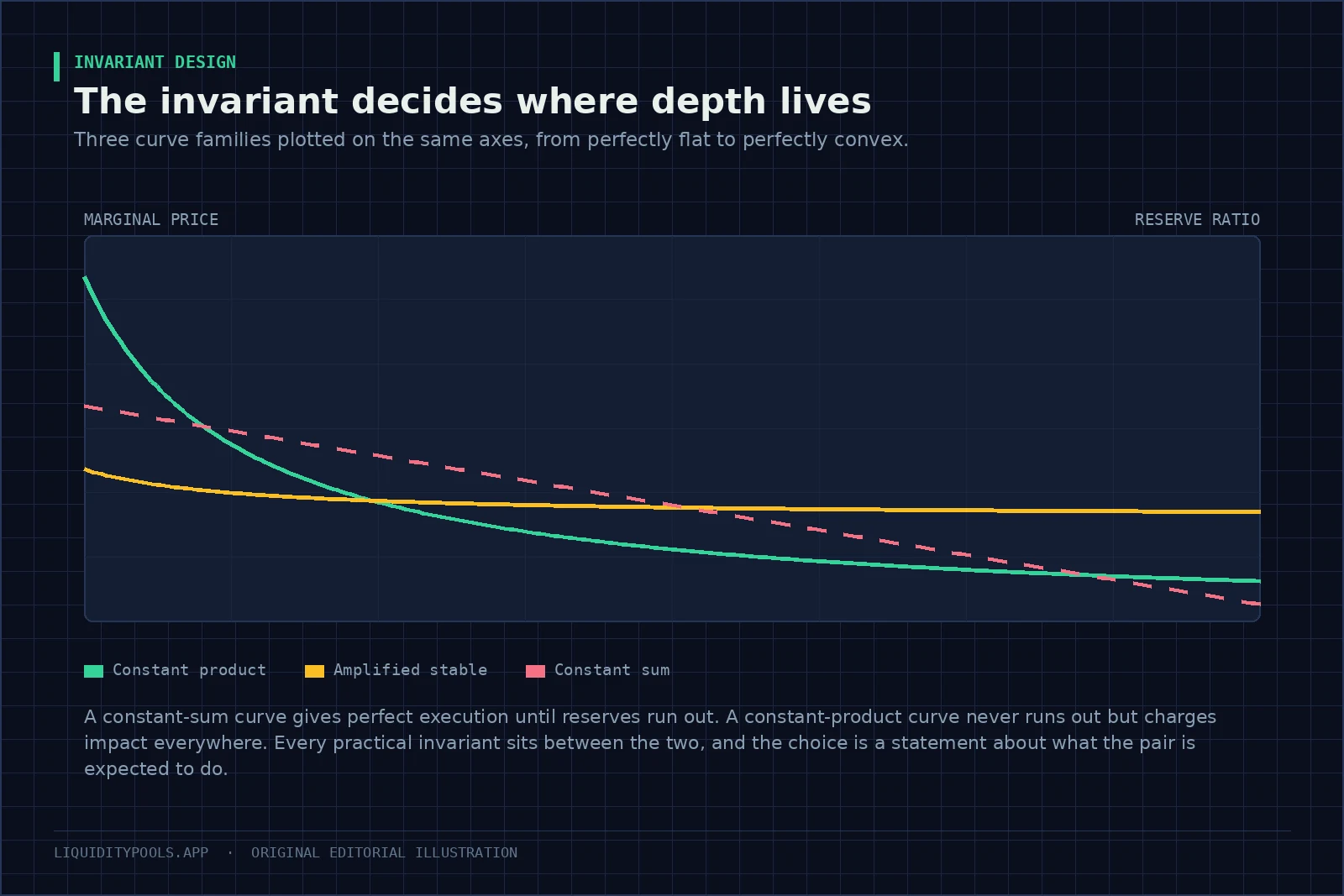
Key point: Curvature is what a pool charges for the chance that its price is wrong. A flat curve gives traders excellent fills while the assumption behind it holds, and offers no protection when it breaks. A bent curve charges a little on every trade and never lets the pool be emptied. Choosing between them is choosing which of those risks you want to be paid for.

The flat one: perfect fills, no defence

The simplest rule is a constant-sum invariant — the quantity a pool keeps fixed through every trade. Here it holds the two balances added together at a fixed number.

$$x + y = k$$

Where:

• $x$ and $y$ are the two token balances.
• $k$ is the total the pool keeps level.

Because the sum never changes, the price never changes either. One for one, whatever the balances look like. Trades have no price impact at all, only the fee, which sounds ideal.

It fails as soon as the real price moves. If one token is worth 95 cents elsewhere, traders buy the whole supply of the other one at par. The pool ends up holding only the weaker token, and nothing in the rule could stop them.

Standalone constant-sum pools are rare for that reason. The rule shows up as an ingredient in mixed designs, contributing flatness near the ratio the pair is supposed to hold^[3].

The workhorse: always solvent, always charging

The rule behind most pools holds the two balances multiplied together at a fixed number^[1].

$$x \cdot y = k$$

Where:

• $x$ and $y$ are the balances.
• $k$ is the product the pool refuses to let fall.

Multiplying rather than adding changes the behaviour completely. As one balance shrinks toward zero, the other must grow without limit, so no sequence of trades can fully drain the pool^[7]. There is always a price at which it will trade.

The price you pay reflects that. Before fees, the shortfall against the quoted price depends only on how big your order is next to the pool:

$$\text{impact} = \frac{\Delta x / x}{1 + \Delta x / x}$$

Where:

• $\Delta x$ is your order size.
• $x$ is the pool’s balance of what you are paying in.
• The result is the share of output you lose against the quoted price, before fees.

Pay in an amount equal to 10% of that balance and you receive about 9.1% less than the quoted price implies. Pay in half the balance and you receive a third less. That rising cost is the mechanism that keeps inventory available at every price. The full derivation is in The Constant Product Formula.

The compromise: flat where it matters

Mixed designs blend the two. Curve’s StableSwap is the best-known, and its author describes it as adding a scaled constant-sum term to the constant-product rule^[3].

Near balance it behaves almost like the flat rule, so a pegged pair trades with almost no price impact. As the balances skew, it bends toward the multiplying rule, so the pool stays solvent.

A single setting, the amplification coefficient, decides where that handover happens. Turn it up and the middle gets flatter and the edges sharper. Turn it down and you approach an ordinary pool.

The trade-off cannot be designed away. Flatness gives efficient fills while the peg holds, and makes the pool absorb the weaker token when the peg breaks. See Stablecoin Liquidity Pools for what that looks like in practice.

Concentration is a separate choice

Here is a point that trips people up. Concentrated liquidity is not a fourth curve. It is the same multiplying curve, shifted so the balances run out at bounds you chose^[2].

Inside your band, the same money backs far more depth. Outside it, you hold one token and quote nothing at all.

Bin designs push the idea further. Each bin holds liquidity at one fixed price, so a trade inside a bin has no price impact, only the fee. The price steps rather than slides as bins empty^[10].

So there are two independent decisions. Which curve family, and how tightly concentrated within it. See Types of Liquidity Pools.

What the shape costs you

Curvature and what arbitrage takes from you are linked directly. The rate at which arbitrage drains a pool grows with how much inventory the curve hands over per unit of price move^[4].

Skip the algebra and keep the intuition. A flatter curve hands over more inventory for the same price move, because it barely adjusts its quote until the balances have shifted a long way. Research on curvature reaches the same split: flat curves suit assets whose value is roughly fixed, and more curved ones protect providers better when traders know more than the pool^[6].

Curve	Price impact for traders	How fast your holdings flip	What goes wrong
Flat sum	None, until one side is empty	Immediately and completely	You hold only the weak token
Amplified	Almost nothing near balance	Fast near balance	You absorb a token that broke its peg
Constant product	Rises with order size	Gradual, symmetric	The ordinary divergence from holding
Concentrated	Low inside the band, for its size	Fast inside the band	Complete conversion at the edge

Why fees and curves are so often mismatched

The curve decides how much value leaks out. The fee decides how much the pool charges for it. Those two numbers are usually set by different people at different times, and they frequently disagree.

A flat amplified curve on a pair whose peg is genuinely solid can run on one basis point — a hundredth of a percent — because almost nothing leaks. Put the same curve on a shakier pair and that fee is far too low. The pool absorbs the dislocation at close to par and charges very little for it.

It happens in reverse too. A 1% fee on an ordinary pool holding two stablecoins charges far more than the curve needs, so the volume simply goes somewhere cheaper.

Setting the fee is a genuine trade-off. Higher fees compensate providers for arbitrage, but they also make the pool’s price less accurate and push away ordinary flow^[8].

The useful test is not what neighbouring pools charge. It is whether the fee has kept up with how much the pair actually moves. If volatility has doubled and the fee has not, the pool is underpriced. Closing that gap is what adjustable fees are for; see Dynamic Fees in AMMs.

How to read an unfamiliar curve

1. Find where it is flat, and name the assumption. Flatness always prices a belief. Work out what that belief is and whether you share it.
2. Find the corner. Every design has a point where behaviour changes sharply. Locate it before you deposit, not after.
3. Simulate a 10% dislocation. Work out what you would be holding. If the answer is uncomfortable, the pool is not for you.
4. Ask who can change the settings. An amplification coefficient under governance control is a live variable, not a constant. DeFi governance is often more concentrated than it looks, so check who actually holds the votes, and whether a delay applies before a change takes effect^[9].
5. Compare quoted depth against an ordinary pool of the same size, for a trade you would actually make.
6. Check whether concentration is layered on top, because that changes the answer to every question above.
7. Size the position against the failure, not against the yield.

A curve that answers all seven cleanly is usually a small variation on one of the three shapes. If you cannot answer the second or fourth, the main risk is not the curve. It is the people who can change it. Weighted pools are the classic variation — the product rule with a tunable weight on each token^[5] — covered in Balancer Weighted Pools.

To see how far a constant-product, weighted or concentrated position falls behind simply holding at any price — its impermanent loss — use the impermanent loss calculator.

References

1. Uniswap v2 Core (Adams, Zinsmeister & Robinson, 2020)
2. Uniswap v3 Core (Adams et al., 2021)
3. StableSwap - efficient mechanism for Stablecoin liquidity (Egorov, 2019)
4. Automated Market Making and Loss-Versus-Rebalancing (Milionis et al., 2022)
5. A non-custodial portfolio manager, liquidity provider, and price sensor (Balancer whitepaper, Martinelli & Mushegian, 2019)
6. When does the tail wag the dog? Curvature and market making (Angeris, Evans & Chitra, 2020)
7. Improved Price Oracles: Constant Function Market Makers (Angeris & Chitra, 2020)
8. Optimal Fees for Geometric Mean Market Makers (Evans, Angeris & Chitra, 2021)
9. DeFi risks and the decentralisation illusion (Aramonte, Huang & Schrimpf, BIS Quarterly Review, December 2021)
10. Liquidity Book DLMM: Primer (LFJ documentation)